SelectKBest | POC - atul5001/SelectKBest-Feature-Selection GitHub Wiki
- TAO engineers spend extra efforts tuning a Correlated model for relevant features.
- Reason: In many cases relevant tag(s) having low correlation scores do not rank up in the feature list.
-
SelectKBest Feature Selection:
- Methodology to identify the logically related TAGS with Target tag.
- Select the best features using a Statistical method that checks for significance along with linear relationship among the tags.
- All datasets extracted and used for these experiments were based on CV models in QA and PROD.
- CV models on the platform have a pre-existing trained model with suitable WB features.
- This was used as the starting point of this exercise. The algorithm will be tasked with proposing a sub-set of features that improves the overall quality of the model (based on KPIs listed below).
- The PROD environment has a large number of CV models. When identifying suitable candidates for experimentation, tags were selected based on the following criteria:
- The tag should have WhiteBOX(WB) features or best-correlated features used for modeling.
- The features proposed should match the most extent of WhiteBOX Features.
- Additional features proposed should improve the model's performance power.
- We want to compare the Insample and Outsample:
- Mean Absolute Error (MAE)
- Root Mean Squared Error (RMSE)
- R2 Score
- Increase in R2 Score and Decrease in MAE/RMSE is the key pattern to look out for after the methodologies have been applied.
- The initial POC/experiment was performed on a set of top 100 correlated features comprising the WhiteBOX features.
- Had concerns about doing this at scale.
- Tried this mini-batch approach of 100 features and found scores were consistent with the full batch.
- However, it is unclear why this is the case?
- Logically explained below.
- However, it is unclear why this is the case?
- The situation it does not work well is the situation when distributions are not gaussian. Indeed, more gaussian the distributions are,the better this approach works.
- Does ATPS + SelectKBest sounds good?
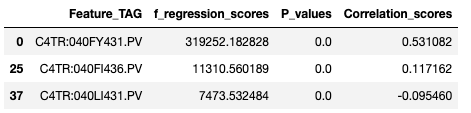
SelectKBest identifies the highly contributing features according to "k" highest scores.
- f_regression scores
- It provides us the ability to execute Correlation and F-Test simultaneously for the provided pool of features against the associated target tag.


- Pearson correlation measures a linear relation and can be highly sensitive to outliers.
- It cannot distinguish between independent and dependent variables. Therefore, also if a relationship between two variables is found, Pearson’s r does not indicate which variable was ‘the cause’ and which was ‘the effect’.
- It assumes that there is always a linear relationship between the variables which might not be the case at all times.
- It can be easily misinterpreted as a high degree of correlation from large values of the correlation coefficient does not necessarily mean a very high linear relationship between the two variables.
-
Univariate linear regression tests returning F-statistic and p-values.
-
Quick linear model for testing the effect of a single regressor, non-sequentially for many regressors.
-
This is done in 2 steps:
-
The cross correlation between each regressor and the target is computed, that is, ((X[:, i] - mean(X[:, i])) * (y - mean_y)) / (std(X[:, i]) * std(y)) using r_regression function.
-
It is converted to an F score and then to a p-value.
-
-
f_regression is derived from r_regression and will rank features in the same order if all the features are positively correlated with the target.
Note: however that contrary to f_regression, r_regression(represent's Pearson correlation results) values lie in [-1, 1] and can thus be negative. f_regression is therefore recommended as a feature selection criterion to identify potentially predictive features for a downstream classifier, irrespective of the sign of the association with the target variable.
-

-
In the above reference, the kind of F-Test being performed is the ANOVA test where, we determine the variance of the features and how how well this feature discriminates between two classes.
-
What makes F1 better than F2?
- The distance between means of class distributions on F1 is more than F2. (𝑑𝑖𝑠𝑡𝑎𝑛𝑐𝑒_𝑏𝑒𝑡𝑤𝑒𝑒𝑛_𝑐𝑙𝑎𝑠𝑠𝑒𝑠)
- The variance of each single class according to F1 is less than those of F2. (𝑐𝑜𝑚𝑝𝑎𝑐𝑡𝑛𝑒𝑠𝑠_𝑜𝑓_𝑐𝑙𝑎𝑠𝑠𝑒𝑠)
- Now we can easily say 𝑑𝑖𝑠𝑡𝑎𝑛𝑐𝑒_𝑏𝑒𝑡𝑤𝑒𝑒𝑛_𝑐𝑙𝑎𝑠𝑠𝑒𝑠/𝑐𝑜𝑚𝑝𝑎𝑐𝑡𝑛𝑒𝑠𝑠_𝑜𝑓_𝑐𝑙𝑎𝑠𝑠𝑒𝑠 is a good score! Higher this score is, better the feature discriminates between classes.
-
F-Test technique involved, uses ANOVA (Analysis of Variance) methodology to test the significance of the features.
- Assumptions of ANOVA:
- The experimental errors of your data are normally distributed.
-
Equal variances between treatments.
- Homogeneity of variances
- Homoscedasticity
-
Independence of samples
- Each sample is randomly selected and independent.
- Assumptions of ANOVA:
-
F-Regression may throw garbage value if the distribution of a feature tag/sensor is non-normal, but
-
For large N(sample size):
- The assumption for Normality can be relaxed.
- ANOVA not really compromised if data is non-normal.
-
For large N(sample size):
-
Assumption of Normality is important when:
- Very small N(sample size).
- Highly non-normal.
- Small effect size.
-
Simple Chart explaining the same:

End Note: With very large sample size, the assumption on Normality in ANOVA is flexible with non-normal distributions and the F-Test technique is considered to be robust on these distributions.
Source:
- https://sites.ualberta.ca/~lkgray/uploads/7/3/6/2/7362679/slides_-_anova_assumptions.pdf
- https://www.psicothema.com/pdf/4434.pdf
- https://statistics.laerd.com/statistical-guides/one-way-anova-statistical-guide-3.php#:~:text=As%20regards%20the%20normality%20of,the%20Type%20I%20error%20rate.
-
To handle edge cases:
   # Scaling
   scaler = StandardScaler()
   scaled_features = scaler.fit_transform(feature_df)
   scaled_features_df = pd.DataFrame(scaled_features, index=feature_df.index, columns=feature_df.columns)

   # Checking if a Feature Tag is Normally Distributed or not as per the ANOVA Assumption
   for col in scaled_features_df.columns:
       # Checking Uniformity
       x = kstest(scaled_features_df[col],"norm")
       p_val = x[1]
       # Now checking if p_val is greater than 0.05
       if p_val > 0.05: # non-uniform
           # Applying Box-Cox transformation
           fitted_data, fitted_lambda = stats.boxcox(scaled_features_df[col])
           scaled_features_df[col] = transformed_data
       else:
           pass
def univariate_methodology(feature_df,target_df,max_features_user_wants,scoring_function):

    '''
    Input:
        - feature_df: dataframe consisting features data
        - target_df: dataframe containing target data
        - max_features_user_wants: Maximum feature to be shortlisted from the CORRELATED pool of features

    Execution:
        - SelectKBest requires the dataset to be in Numpy characteristic.
        - Then we eventually specify the TOP features to choose and using which score_function
        - Then we return the final selected feature names which we can use to create a new model.

    Return:
        - Feature List Names
        - Target Name
        - A Dataframe comprising Correlation Scores and P-Values for each feature
    '''
    start_time = datetime.now()
    features = feature_df.values
    target = target_df.values.ravel()
    # target = target.astype('int')
    # print('Feature shape:',features.shape)
    # print('Target shape:',target.shape)

    # feature extraction
    print('User has asked for maxx {} features'.format(max_features_user_wants))
    test = SelectKBest(score_func = scoring_function, k=max_features_user_wants)
    '''
    score_func: Function taking two arrays X and y, and returning a pair of arrays
                (scores, pvalues) or a single array with scores.

    f_regression: F-value between label/feature for regression tasks.
    The goal of the F-test is to provide significance level. If you want to make sure the features your are
    including
    are significant with respect to your 𝑝-value, you use an F-test.
    If you just want to include the 𝑘 best features, you can use the correlation only.
    Ref:
        - https://stats.stackexchange.com/questions/204141/difference-between-selecting-features-based-on-f-regression-and-based-on-r2
        - https://scikit-learn.org/stable/modules/generated/sklearn.feature_selection.f_regression.html#sklearn.feature_selection.f_regression

    Alternatively we can use:
        - mutual_info_regression: Mutual information for a continuous target.
        Estimate mutual information for a continuous target variable.
        Mutual information (MI) between two random variables is a non-negative value, which measures the
        dependency between the variables. It is equal to zero if and only if two random variables are independent,
        and higher values mean higher dependency.

        The function relies on nonparametric methods based on entropy estimation from k-nearest neighbors
        distances.

    ref: https://scikit-learn.org/stable/modules/generated/sklearn.feature_selection.SelectKBest.html#sklearn.feature_selection.SelectKBest
    '''

    fit = test.fit(features,target)
    feature_scores = fit.scores_[fit.get_support()]
    print('Completed SelectKBest function')

    mask = test.get_support()
    new_features = feature_df.columns[mask]
    prep_df = pd.DataFrame()
    prep_df['Columns'] = feature_df.columns
    prep_df['{}_scores'.format(scoring_function.__name__)] = fit.scores_
    prep_df['P_values'] = fit.pvalues_
    out_list = []
    for column in feature_df.columns:
        corr_tuple = pearsonr(feature_df[column], target)
        out_list.append(corr_tuple[0])

    prep_df['Correlation_scores'] = out_list
    # print(fit.scores_)
    print('Completed Seleting new features.')
    end_time = datetime.now()
    print('Total time taken for SelectKBest execution: {}'.format(end_time - start_time))
    return new_features,target,prep_df
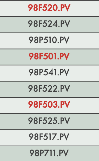
- Target Tag: 98P503.MV
- Tag in PRD Environment
- Results are documented in the slide pack also.
| Correlated Features | SelectKBest Features | WB Features | LIVE Model KPI | SelectKBest Model KPI |
|---|---|---|---|---|
 |
|
|
Insample Metrics :
|
Insample Metrics :
|
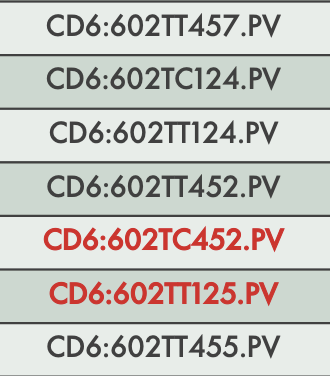
- Target Tag: CD6:602TC457.PV
- Tag in QA Environment
- Results are documented in the slide pack also.
| Correlated Features | SelectKBest Features | WB Features | LIVE Model KPI | SelectKBest Model KPI |
|---|---|---|---|---|
 |
|
|
Insample Metrics :
|
Insample Metrics :
|
For more results, please refer:
- PPT: Feature Selection Deck
- The other TAGS included for proving the concept as part of POC experiments:
-
CD6:602PC037.PV CD6:602TT108.PV MLO:021F064.MV MEOD:093P007.OP P4049_ID2_OP 98P503.MV 114FICA034.MV MLO:021F052.MV LS41243_AO4_OP HV8:008PC113.OP HDS5:86PT122.PV CD6:602TC457.PV CD6:608FC005.OP
-
- Since, SelectKBest uses f_regression scoring function, which uses F-Test/ANOVA Test to identify the significance of relationship between feature and target, this whole process when combined is a univariate process of feature selection.
- For each feature, the above mentioned formula of 𝑑𝑖𝑠𝑡𝑎𝑛𝑐𝑒_𝑏𝑒𝑡𝑤𝑒𝑒𝑛_𝑐𝑙𝑎𝑠𝑠𝑒𝑠/𝑐𝑜𝑚𝑝𝑎𝑐𝑡𝑛𝑒𝑠𝑠_𝑜𝑓_𝑐𝑙𝑎𝑠𝑠𝑒𝑠 is calculated and respective F-Score is obtained from the F-table.
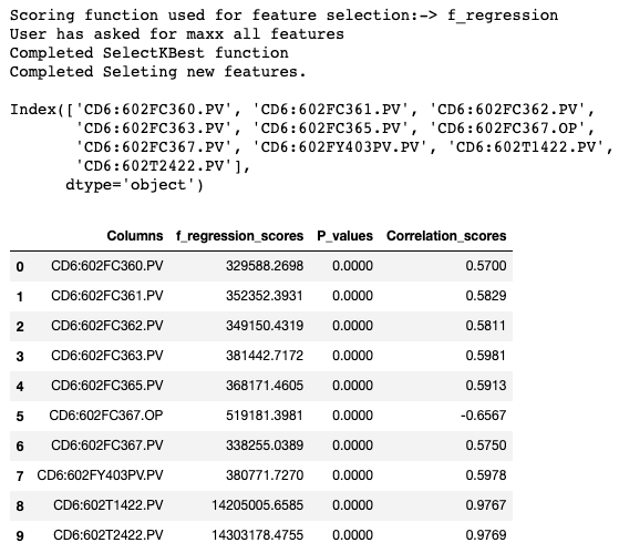
- We performed a small experiment on a piece of equipment, where we chose:
-
Set of first 10 features, and ran SelectKBest to identify the scores.
-
Set of next 10 features, and ran SelectKBest to identify the scores.
-
Set of final 100 features, and ran SelectKBest to identify the scores.
-
And, now if we try to see some common features from all the 3 sub-experiments, we find:
-
This proves the resulting experiment that the results of mini-batch execution of f_regression matches with full batch execution results.
-


| **** | SelectKBest Methodology | Pearson Correlation Methodology |
|---|---|---|
| Computationally Efficient? | Equivalent | Equivalent |
| Better Performance? | Equivalent | Equivalent |
| Effective in Reducing Training Time? | Equivalent | Equivalent |
| More Granular resulting methodology? | ✅ As, it is more statistical and free from any bias. | Depends only on the linear behaviour, but not on statistical behaviour. |
-
Mutual Information Regression.
- https://stats.stackexchange.com/questions/20341/the-disadvantage-of-using-f-score-in-feature-selection
- Reveals Mutual information among features.
- Computationally expensive.
- Time expensive process.
- Requires more narrowed features to target, unit/sub-unit level features.
TAG: MLO:021F064.MV
- Moerdijk
- Plant id: 0635EC1E-533F-4FE0-8C46-295F41B28F48
- Run SelectKBest on the whole plant
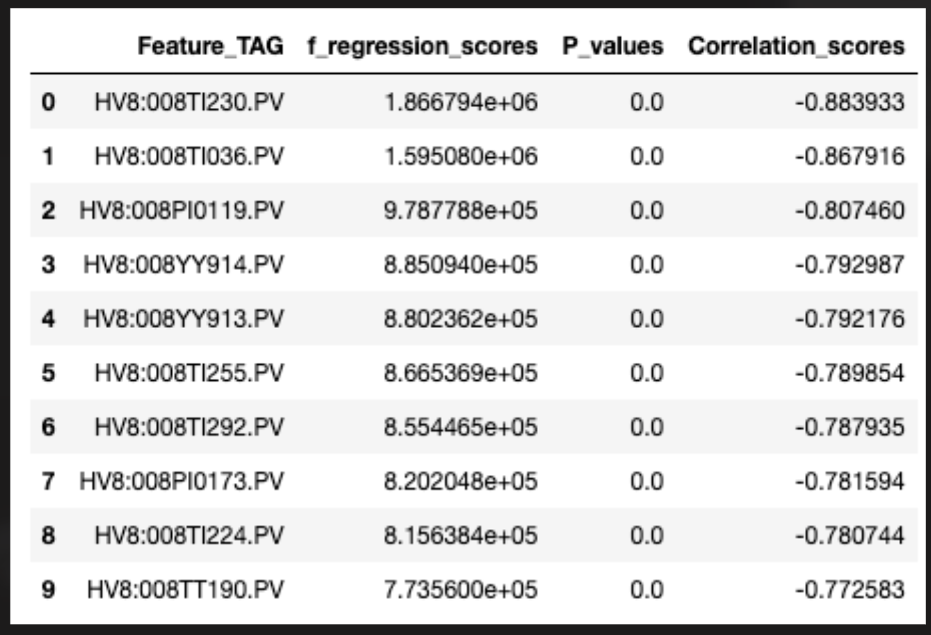
- Document top 10 features as per f_regression score, and create a model using the same

TAG: HV8:008PC113.OP
- Pernis
- Plant id: 3A158E3B-AC18-46FA-9720-04917B461035
- Run SelectKBest on the whole plant.
- Document top 10 features as per f_regression score, and create a model using the same.
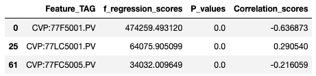
TAG: CVP:77FC5005.OUT
- Pernis
- Plant id: BCB4D346-0713-4E53-8BAF-1A8FF6DBBCA7
- Tag outside of POC

- WB Features in SelectKBest features?
- WB Features in Correlation features?
- None of the WB Features appeared in Correlated features.
- None of the WB Features appeared in Correlated features.
TAG: C4TR:040PC431.OP
- Pernis
- Plant id: 20BDA776-6197-4CCD-BF37-70149E597DF8
- Tag outside of POC
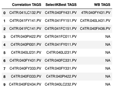
- WB Features in SelectKBest features?
- WB Features in Correlation features?
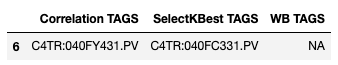
- The SelectKBest proposed features are mostly from the same drawing (PID diagram)
- Some of the features selected could have been included if Correlation would have selected them.
- Results are somewhat similar/little bit improved than the Correlation methodology.
- As per multiple conversations with @toluogunseyeatshell:
- We should put it in QA and check out how much it improves as the performance issue with respect to correlation is taken care of.
- Test it out on more number of TAGS and keep TAO in loop with respect to the features proposed by SelectKBest
Testing Workbook: https://my.shell.com/:x:/g/personal/disha_soni_shell_com/EVW9ZCKnNNtLhwbc4MuntdYBBvzM5gPhH1p0_0zetYY_9g?email=Atul.Mishra%40shell.com&e=tkOENo
-
SelectKBest := 'f-regression' performs almost similar or a slightly better than Correlation, but not that significant enough to conclude it as a break-through methodology.
- Technical reason being that it is a univariate approach which does involves Correlation and that's why similar performance and features are observed.
- Also, every-time the methodology consumes more than 11k+ features, Correlation tends out to be the driving factor for feature selection.
- Most of the WB models tested had features belonging to the same UNIT and are chosen irrespective of their correlation value.
- Large number of non-GREEN models are also LIVE with reason:
- The predicted difference offset is very low, meaning prediction trend matches the OP signal for a larger amount of time. Hence made the model LIVE.
- This gives us the idea to work on AutomatedLIVE model scenario improvement.
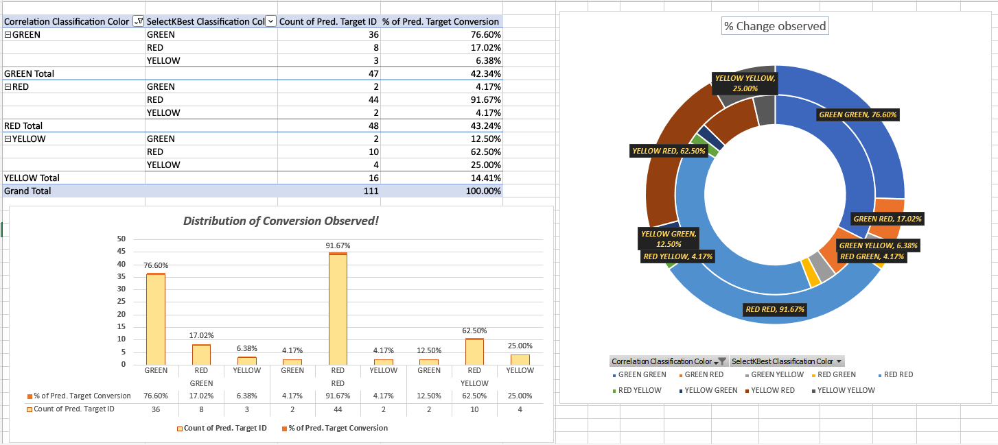

- Testing involved 110+ tags.
- Testing Results summarised in the below workbook:
- SelectKBest Wiki Page with logic + POC + implementation + Testing on PROD Data remarks:
- SelectKBest Feature Selection · sede-x/shell-platform Wiki (github.com)
- Observations documented.
- PPT while proposing the POC:
- Final Comments observed after testing:
- Given that SelectKBest works better than Correlation theoretically, it underperforms due to high number of tags considered while running the methodology.
- While doing POC, selection of 100 tags were made as UI provides that much only and downloading the data of thousand tags on a minute is not feasible for local system.
- On Average 10k+ features are selected for Correlation/SKB Job since the mapping of Hierarchy happens on Plant level and not on Unit Level.
- This is the same challenge that Correlation logic also faces currently.
- The objective of proposing improved set of TAGS using SelectKBest returns Pearson Correlation Features mostly.
- Evidence that most of the LIVE models consume features belong to the UNIT LEVEL:
- We should look for a way to decrease the number of feature TAGS considered for correlation/skb execution.
a. Possible via C3 mapping.
b. Generalizing TAG Nomenclature.
c. This can help in identifying UNIT LEVEL TAGS.
1. The pool of features considered for Feature Selection strategy needs to be refined more in order to achieve better set of features.
2. SelectKBest strategy works better on the UNIT level hierarchy as the F-Statistic helps in achieving same characteristic feature tags.
- Also, Overall significance of F-statistics helps in identifying model significance. Keeping such features is going to result in a statistically significant model.
3. We should continue with Univariate feature selection methodology of Correlation.
- The feature selection strategy discussed above is helpful in pre-modeling phase, in addition to current correlation based approach, which we recommend to keep as is.
4. Caveat - The results though tested on 100 CV use cases, are reflection of data used for training purposes only. Having a different period of analysis may or may not change the results significantly.